Principal Component Analysis (PCA)

Motivation

When employing regression analysis methods, one often face the problem of multicollinearity. Multicollinearity arises when predictors in our specified linear regression model are linearly dependent (highly correlated) — making it difficult to isolate their individual effects on the response variable. One way of tackling this problem is to apply dimension reduction techniques of which one of them is PCA.

In this guide, we will derive the mathematics behind Principal Component Analysis and demonstrate, through and example, how to obtain the principal component loadings and how to compute the corresponding amount of variance along these loadings.

Finding the First Principal Component

So how would one practically reduce the dimension from \( p \) to \( m < p \)? Well one could simply remove one of the features of the original design matrix \( \mathbf{X} \), right? I mean, that is what we usually do when we accidently included a feature that is highly multicollinear with some other already present feature?

That would however have the effect of losing all the information that exists in this feature we would prefer to include. Another approach would be to project this data onto a lower space using all the features in our data, no matter if they're multicollinear or not, while still trying to capture as much variation as possible. This is precisely what we are going to do.

First, let's center our data \[ \bar{\mathbf{X}} = \frac1n \sum_{i=1}^n \mathbf{x}_{ij} \]

Now, due to the fact that the data is centered, the variance of our projection can be expressed and simplified as \[ \mathrm{Var}(\mathbf{v}^\top \mathbf{x}) = \mathbf{v}^\top \mathbb{E} \left[\mathbf{x}\mathbf{x}^\top\right] \mathbf{v} = \mathbf{v}^\top \Sigma \mathbf{v} \] where \( \Sigma \) is our covariance-variance matrix.

One could now (naively) maximize the variance of this expression by simply solving \[ \max_{\mathbf{v}} \mathbf{v}^\top \Sigma \mathbf{v}, \] but this optimization problem is poorly specified, because then we could simply increase \( \mathbf{v} \) and always find a "better" solution. It is therefore necessary for us to specify a restriction that \( \mathbf{v}^\top \mathbf{v} = 1 \), giving us the following problem \[ \max_{\mathbf{v}} \mathbf{v}^\top \Sigma \mathbf{v}, \quad \text{s.t. } \mathbf{v}^\top \mathbf{v} = 1 \]

This one can fairly easily be solved by formulating a lagrangian such as \[ \mathcal{L}(\mathbf{v}, \lambda) = \mathbf{v}^\top \Sigma \mathbf{v} - \lambda\,(\mathbf{v}^\top \mathbf{v} - 1). \]

Solving \( \nabla_{\mathbf{v}} \mathcal{L} \stackrel{!}{=} 0 \) yields \[ \Sigma \mathbf{v} = \lambda \mathbf{v}. \]

If one looks at twice equation twice, you'll notice that this is actually the eigen decomposition. The eigenvectors \( \mathbf{v}_1, \mathbf{v}_2, \dotsc, \mathbf{v}_p \) of \( \Sigma \) here defines the directions (principal component loadings) along which the data varies the most. Likewise, the corresponding eigenvalues \( \lambda_1 \geq \lambda_2 \geq \cdots \geq \lambda_p \) quantifies how much of the variation is explained by each component. The fact that we can quantify how much of the variation is explained by each component means that we can compute the proportion of variance explained by each component as \[ \mathrm{PVE}_i = \frac{\lambda_i}{\sum_{j=1}^p \lambda_j} \in [0,1] \]

This is all fine and dandy, but if we would like to find more than one principal component we need to make sure that all the principal component loadings are orthogonal to one another. If we did not enforce this constraint as well, then the next principal component will capture variation of which the other components has already captured — effectively capturing less variance in total.

Finding Multiple Principal Components

When finding multiple principal components it's much more handy to go over to matrix notation and instead formulate the objective function as \[ \sum_{j=1}^m \mathbf{v}_j^\top \Sigma \mathbf{v}_j = \mathrm{tr}\!\left(\mathbf{V}^\top \Sigma \mathbf{V}\right). \]

Now to enforce the following two constraints \[ \begin{align*} \mathbf{v}_i^\top \mathbf{v}_i &= 1, && \forall i && \text{(normalization)} \\ \mathbf{v}_i^\top \mathbf{v}_j &= 0, && \forall i \neq j && \text{(orthogonality)} \end{align*} \]

Knowing these constraint, we can reformulate them in matrix form as \[ \mathbf{V}^\top \mathbf{V} = \mathbf{I}_m. \]

This gives us the optimization problem as \[ \max_{\mathbf{V}} \; \mathrm{tr}\ \left(\mathbf{V}^\top \Sigma \mathbf{V}\right), \quad \text{s.t. } \mathbf{V}^\top \mathbf{V} = \mathbf{I}_m. \] which yields the following Lagrangian \[ \mathcal{L}(\mathbf{V}, \Lambda) = \mathrm{tr}\!\left(\mathbf{V}^\top \Sigma \mathbf{V}\right) - \mathrm{tr}\ \left[ \Lambda \left(\mathbf{V}^\top \mathbf{V} - \mathbf{I}_m\right)\right ], \]

Now we do as we did in the case for only one principal component and set the gradient equal to zero, which gives \[ \nabla_{\mathbf{V}} \mathcal{L} = 2\Sigma \mathbf{V} - 2\mathbf{V}\Lambda \stackrel{!}{=} 0 \quad \Longrightarrow \quad \Sigma \mathbf{V} = \mathbf{V}\Lambda. \]

From now on, the eigenvalue decomposition \( \Sigma \mathbf{V} = \mathbf{V}\Lambda \) is precisely what we are going to calculate.

Applying PCA to Simulated Data

Let's now generate some simulated data and apply PCA in practice — for this I will be using Python.

In the first step, we will now generate some data drawn from a (multivariate) normal distribution, and standardize the data so that each feature is distributed as \( \mathbf{x}_j = \mathcal{N}(0,1) \).

import numpy as np

np.random.seed(42) # To make deterministic

mean = np.array([12, 7, 5])
cov = np.array([
    [7, 2.5, 1.5],
    [2.5, 4, 0.5],
    [1.5, 0.5, 3],
])

X = np.random.multivariate_normal(mean, cov, 200)
X = (X - X.mean(axis=0)) / X.std(axis=0)

Plotting this data would give us the following

I'm now going to set the goal of reducing this space from \( p = 3 \) to \( m = 2 \) dimensions. Effectively, we are going to perform the following two tasks

• Find the first two principal components
• Calculate how much of the total variance is explained by these two components

If you understood the explaination in the previous section, we know that the next step is to use the equation \( \Sigma \mathbf{V} = \mathbf{V}\Lambda \) in order to find \( \mathbf{V} = [\,\mathbf{v}_1 \;\; \mathbf{v}_2\,] \). To do this, we first need to calculate the second moment matrix \( \Sigma = \mathbf{X}^\top \mathbf{X} \) and then simply use the built-in algorithm for finding the principal components. We are also going to organize the eigenvectors in descending order according to their corresponding eigenvalues

sigma = X.T @ X
eigenvalues, eigenvectors = np.linalg.eig(sigma)
idx = np.argsort(eigenvalues)[::-1]
eigenvalues = eigenvalues[idx]
eigenvectors = eigenvectors[:, idx] 

If you now print the eigenvalues and eigenvectors which we have stored, you will find \[ \Lambda = \begin{bmatrix} 295.87 & 0 & 0 \\ 0 & 185.87 & 0 \\ 0 & 0 & 118.26 \end{bmatrix}, \qquad \mathbf{V} = \begin{bmatrix} 0.6781 & -0.0324 & 0.7343 \\ 0.5549 & -0.6325 & -0.5404 \\ 0.4819 & 0.7739 & -0.4109 \end{bmatrix}. \]

If we start off by calculating the fraction of variance which will be captured by our first two principal component loadings, we will find that about 80% will be captured \[ \frac{\lambda_1 + \lambda_2}{\sum_{j=1}^{3} \lambda_j} = \frac{295.87 + 185.87}{295.87 + 185.87 + 118.26} \approx 0.80. \]

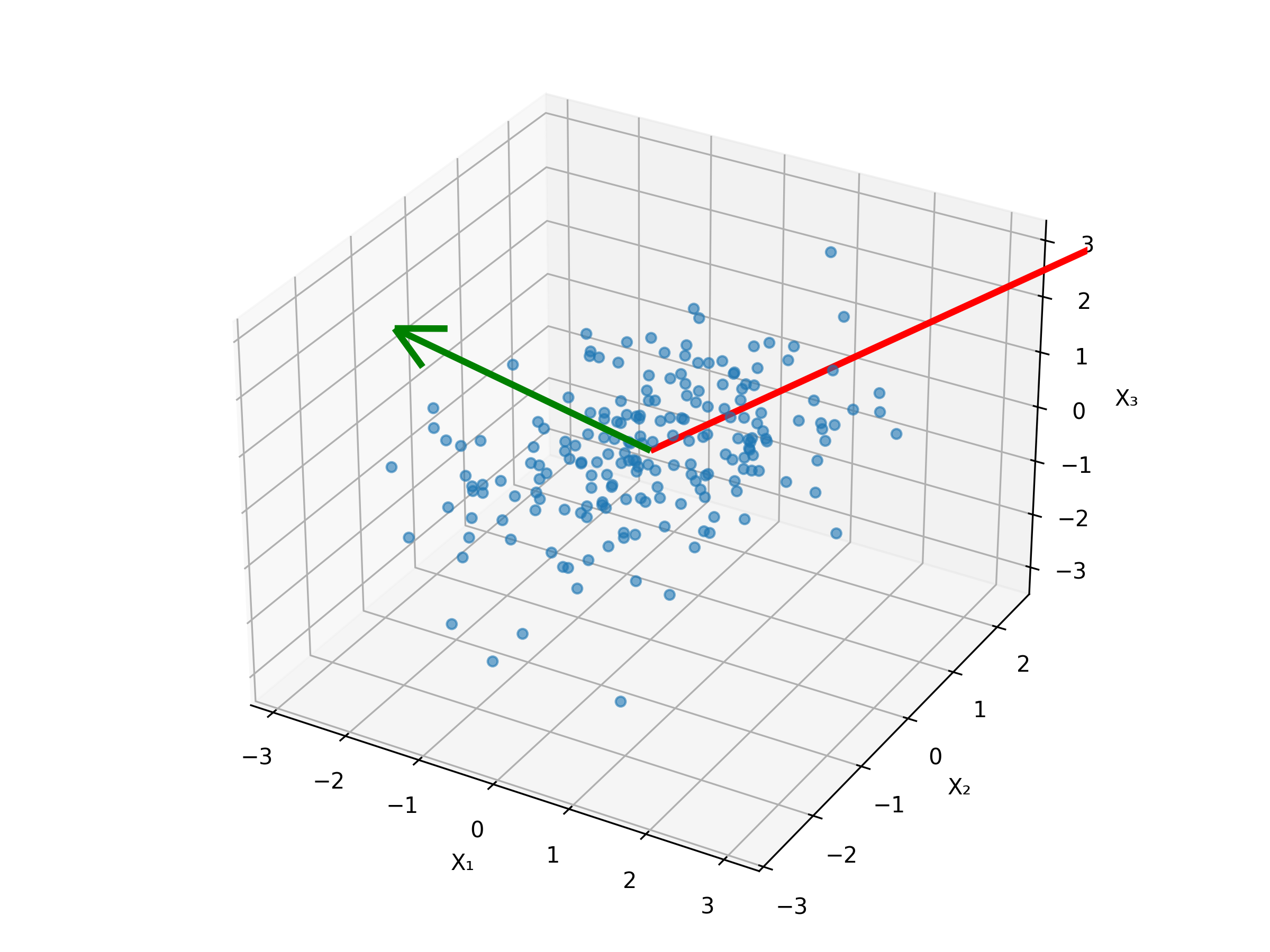
Finally, plotting these two components in the original feature space makes it graphically clear that

• the principal components are orthogonal, and
• that the first principal component points in the direction of the greatest variance.